COMPUTER: FORM TWO: Topic 2 - SPREADSHEET

 Join Our Groups

TELEGRAM | WHATSAPP

Schemes of Work 2024

English Course - Free

Kenya Resources

TOPIC 2: SPREADSHEET

Concept and Terminologies

The Spreadsheet Program

Describe the Spreadsheet Program

A spreadsheet is an interactive computer application for organization, analysis and storage of data in tabular form. Alternatively referred to as a worksheet, a spreadsheet is a file made of rows and columns that help sort data, arrange data easily, and calculate numerical data. Examples of spreadsheet programs are:

• Google sheet
• iWork numbers
• Libre Office
• Lotus 1-2-3
• Lotus Symphony
• Microsoft Excel
• Open Office

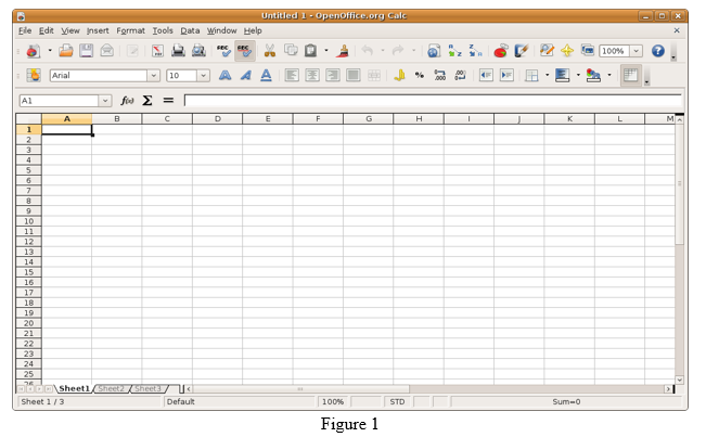
Today Microsoft Excelis the most popular and widely used spreadsheet program (figure 1)

The Spreadsheet Terminology

Explain Spreadsheet Terminology

TERMINOLOGIES USED IN SPEADSHEET (EXCEL)

• Cell - a space created on the spreadsheet / worksheet where a row and column meet
• Cell Address - the label for a cell made up of the column identifier and the row identifier. Example:A1 = column A, row 1 ,C5 = column C, row 5
• Cell Address Box- a rectangular box located at the top left corner of the spreadsheet containing the cell address of the current cell
• Cell Range - a group of cells that are highlighted (selected), or specified for use in a formula. A range includes the first cell address and the last cell address of cells either in a column or down a row. Example: =sum (B4:B10) - identifies all cells in the range from B4 to B10
• Chart / Graph – a visual representation of selected data. Charts help make the data easier to understand and “see”. Use the Chart icon or hit F11 for the chart feature. Some common chart types to choose from are: pie chart, line, column, bar, line etc.
• Current Cell - the cell that is active or selected and has a highlighted border
• Formula - a formula helps you to calculate and analyze data on your worksheet. Formulas contain cell references and mathematical operators (Remember, a function is like a keyword that is part of a formula.

There are 4 steps in creating a formula:

1. select the cell where you want the result of the formula to appear
2. key in the calculation / formula = B5*D5.
3. press Enter to “register” the entry

• Formula Bar - displays the formula of the selected cell. You may edit here.
• Function- is a pre-programmed, frequently used calculation. It is used as part of a formula and usually with a specific range of cells. Eg. = Sum (B1:B7) ; = Average (D4:D10) or = Avg (D4:D10) ; = Max (C5:C15);= Min (C5:C15)
• Labels – Textual information entered onto a worksheet cell. Could be column or row headings (Price, Quantity) or data entries such as student names.
• Relative Cell Reference - is a cell reference that changes when you copy a formula, or “fill” down a column or across a row. For example, the formula A1+A2+A3 will automatically change to B1+B2+B3 and then to C1+C2+C3 when copied or filled to those cells on the worksheet
• Value – Numeric information entered onto a worksheet cell. A value is any “raw” / unformatted number you enter, or results from a calculation on the spreadsheet
• Workbook - contains sheets of different types – such as worksheets and chart sheets. Each Excel file is called a workbook. Each workbook is divided into several sheets, with a tab displayed for each. **Always name your worksheet, simply by highlighting “Sheet 1” and typing new name.
• Worksheet - consists of rows (across) and columns (down) - like a blank sheet of graph paper. In a spreadsheet application; rows are numbered and columns are labeled A, B, C, D etc. An entire Spreadsheet worksheet could contain 256 columns across and 65,536 rows down.

Outline the Uses of Spreadsheet Program

Outline the Uses of Spreadsheet Program

The list of uses for spreadsheet software is endless. However the following are some of them;

• Modelling and Planning
• Household Finance Planning
• Business Accounts and Budgeting
• Invoices
• Wages
• Predictions / Simulations
• Calculations e.g. Adding, Subtracting, etc.
• Break even analysis
• Statistical analysis
• Creating Graphs e.g. bar chart, pie chart.
• Collect data from different sources e.g. phone number, prices.
• Explore and interpret data in order to draw conclusions for business

THE ADVANTAGES OF SPREADSHEETS

• Spreadsheets are preferable to manual calculation and recording of data for a variety of reasons, one very obvious reason is the unlimited space allowed to the user by the ‘spreadsheet’, hence the name.

Other Advantages Include:

• Calculations are correct
• Calculations are completed automatically
• Information is organized and easy to access
• Information is easy to edit if a mistake has been made by retyping or using ‘undo’
• Data can be easily sorted and filtered
• Data can be quickly analyzed
• Reports can be made more visual by using charts and graphs

Starting Ending Spreadsheet Program

Start a Spreadsheet Program

Start a Spreadsheet Program

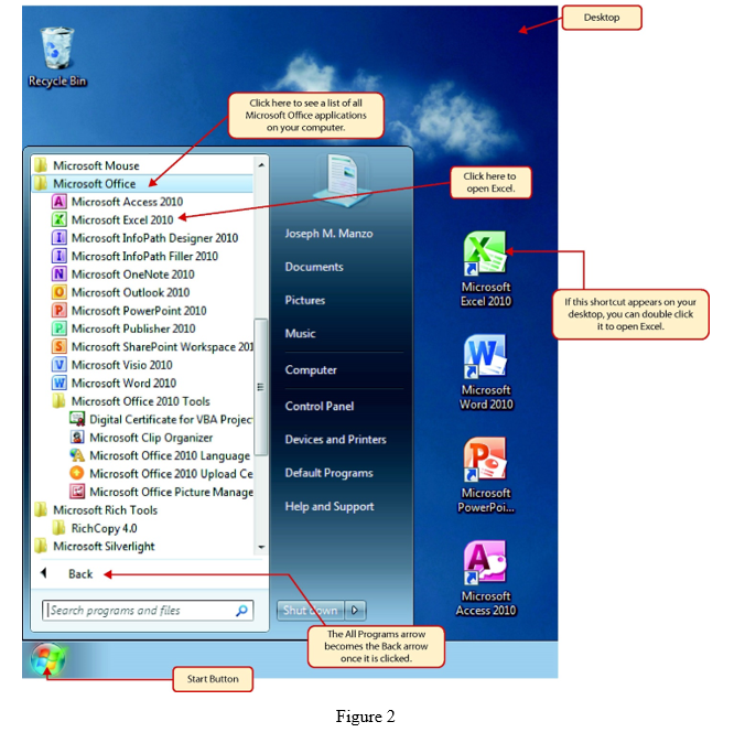
Microsoft excel is one of the most popular spreadsheet processing programs supported by both Mac and PC platforms. The following steps will guide you in starting the Excel application.

• Click the Start button on the lower left corner of your computer screen.
• Click the All Programs arrow at the bottom left of the Start menu.
• Click the Microsoft Office folder on the Start menu. This will open the list of Microsoft Office applications.
• Click the Microsoft Excel 2010 option. This will start the Excel application

Create a Workbook

Create a Workbook

Once Excel is started, a blank workbook will open on your screen. A workbook is an Excel file that contains one or more worksheets (sometimes referred to as spreadsheets). Excel will assign a file name to the workbook, such as Book1, Book2, Book3, and so on, depending on how many new workbooks are opened. Figure 3" shows a blank workbook after starting Excel.

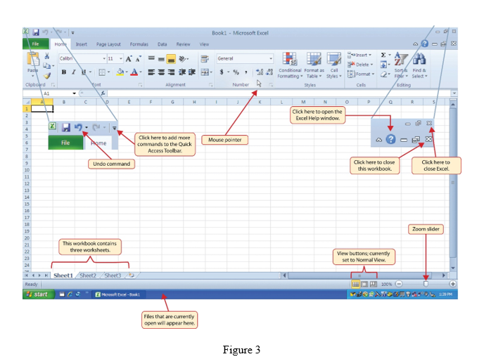
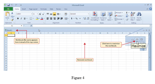
Your workbook should already be maximized (or shown at full size) once Excel is started, as shown in Figure 3 "Blank Workbook". However, if your screen looks like Figure 4 "Restored Worksheet" after starting Excel, you should click the Maximize button, as shown in the figure.

Open a Worksheet

Open a Worksheet

By default, Excel will remember your last modified worksheet as you exit your Excel program every time, and when you open your workbook next time, this sheet will be displayed first.

The following below are steps to open;

1. Click File > Open > Computer > Browse.
2. To only see files saved in the xlsx or Open Document Spreadsheet
3. Find the file you want to open, and then click Open.

Note: When you open an Open Document Spreadsheet file in Excel, it might not have the same formatting as it did in the original application it was created in. This is because of the differences between applications that use the Open Document Format.

Entering and Editing Data

Enter Data in Worksheet

Enter Data in Worksheet

There is more than one way to enter data into an Excel worksheet. Sometimes we stick to typing directly into cells, but there are different ways to enter data which can speed up your data entry work.

1. Type directly into a cell and add your data. You know a cell is active as it is highlighted with a darker border as in figure (5)
2. Use the formula bar. This is located under the ribbon. Type your data directly into the formula bar and press enter. You can navigate around the worksheet by typing the cell number directly into the Name box (located above the Column headings A – Z) as in figure (6)
3. Make the most of auto complete. Excel will try to help you speed up your data entry by guessing what you are typing based on what’s in your worksheet. If the auto correct option is right for you, just press enter as in fig (7)
4. Copy and paste – you may have cells that you can copy and paste data within the same worksheet – it can save you time formatting a sheet, or you can copy data to another worksheet within the workbook.
5. Let Auto fill do the work. Auto fill options can complete series of data, whether it is text or numbers. This saves lots of data entry when setting up worksheets, or entering data.

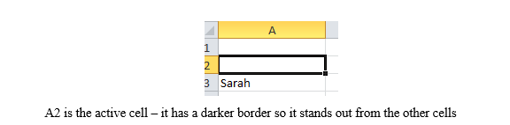
figure 5

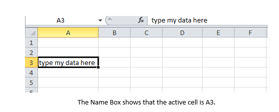
figure 6

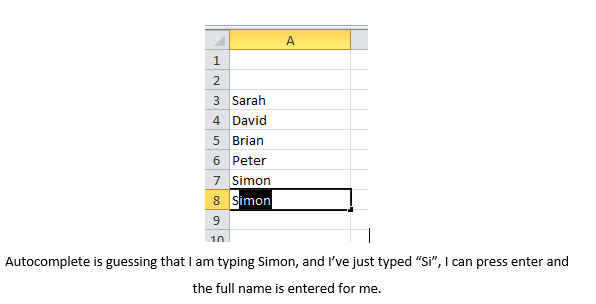
figure 7

Formatting Data in a worksheet

Formatting worksheet (or sheet) data is easier than ever. You can use several fast and simple ways to create professional-looking worksheets that display your data effectively. For example, you can use document themes for a uniform look throughout all of your 2007 Microsoft Office system documents, styles to apply predefined formats, and other manual formatting features to highlight important data.

Data Manipulation

Data manipulation is the process of changing data in an effort to make it easier to read or be more organized.

For example, a log of data could be organized in alphabetical order, making individual entries easier to locate.

Data manipulation is often used on web server logs to allow a website owner to view their most popular pages as well as their traffic sources. Users in the Accounting field or other fields that work with numbers often manipulate data to figure out costs of products, trends in sales, potential tax obligations, or how well merchandise is selling per week or month.

Stock market analysts are frequently using data manipulation to predict trends in the stock market and how stocks might perform in the near future. Computers may also use data manipulation to display information to users in a more meaningful way, based on code in a software program, web page, or data formatting defined by a user.

The Mathematical Operators

Identify Mathematical Operators

Operators specify the type of calculation that you want to perform on the elements of a formula, like addition, subtraction, multiplication or division. There is a default order in which calculations occur, but you can change this order by using parentheses

Different Types of Operators in Excel

Types	Character	Operation	Example
Arithmetic	+(plus sign)	Addition	=A2+B3
	-(minus sign)	subtraction or negation	=A3-A2 or -C4
	*(asterisk sign)	multiplication	=A2*B3
	/	division	=B3/A2
	%	percent(dividing by 100)	=B3%
	^	exponentiation	=A2^3
Comparison/Logical	=	equal to	=A2=B3
	>	greater than	=B3>A2
	<	less than	=A2<B3
	>=	greater or equal	=B3>=A2
	<=	less or equal	=A2<=B3
	<>	not equal to	=A2<>B3
Text	&	concatenates (connects) entries to produce one continuous entry	=A2&” “&B3t
Reference	:(colon)	Range operator that includes	=SUM(C4:D17)
	,(coma)	Union operator that combines multiple references into one reference	=SUM(A2,C4:D17,B3
	space	Intersection operator that produces one reference to cells in common with two references	=SUM(C3:C6 C3:E6)

Most of the time, you’ll rely on the arithmetic operators when building formulas in your spreadsheets that don’t require functions because these operators actually perform computations between the numbers in the various cell references and produce new mathematical results. The comparison operators, on the other hand, produce only the logical value TRUE or the logical value FALSE depending on whether the comparison is accurate.

Data manipulation in spreadsheet including the following but not limited to this ;

• creating new data by transforming existing data
• cell references (relative and absolute)
• selecting or highlighting data
• sorting data
• deleting rows or columns of data

CREATE NEW DATA BY TRANSFORMING EXISTING DATA

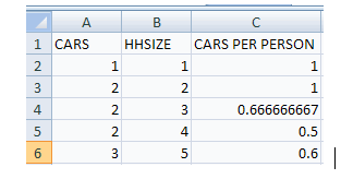
• Suppose you have open a data set with the following information (cars.xls).

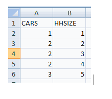
Now additionally create data on cars per person in household. This data will be included in cells C2:C6 under the heading CARS PER PERSON. To do this

• In cell C2 type =A2/B2 (then cell C2 is the entry in A2 divided by that in B2)
• Cut and paste to change the remaining entries in column C. Highlight cell C2 and copy by CTRL-C or by Edit / Copy. Then highlight cells C3:C6 and paste by CTRL-V or by Edit / Paste.
• Finally in cell C1 type CARS PER PERSON.

The ability to manipulate data like this is a great attraction of spreadsheets.

REFERENCES

• Cell reference examplesare;
• Cell B2 is the entry in column B and row 2.
• Cells B2:C10 are the entries from column B row 2 in the top left to column C row 10 in the bottom right. This is 2 columns times 9 rows yielding 18 entries.
• Cell references are most often relative but can also be absolute. Absolute cell references have the prefix $. For example, B2:C10 is a relative cell reference while $B$2:$C$10 is an absolute cell reference.

CELL

Relative cell references can change after copying the cell references to a new location. For example, if D2 = B2+C2 then if we copy cell D2 to D3 (move down one cell) the new cell is D3 = B3+C3.

Absolute cell references do not change after copying the cell references to a new location. For example, if D2 = $B$2+$C$2 then if we copy cell D2 to D3 (move down one cell) the new cell is D3 = $B$2+$C$2.

Cell references can be part relative and part absolute For example, $B2 is absolute column B and relative row 2, while B$2 is relative column B and absolute row 2. Cell references can be to a different worksheet in the current workbook For example, Sheet name! B2:C10 or Sheet name !$B2:$B10. Cell references can be to a different workbook For example, (Workbook name) Sheet name B2:C10 or (Workbook name) Sheet name! $B2:$B10.

SELECTING OR HIGHLIGHTING DATA

• Many Excel commands involve selecting or highlighting data. Do this by

• Click on the first entry in the array.
• Depress the shift key and keep it depressed
• Scroll down to the last entry in the array you want to highlight
• Click on this last entry

For long arrays this can require a lot of scrolling. CTRL-down arrow moves automatically to the bottom of an array. CTRL-up arrow moves to the top,. CTRL-right arrow to the right end of the arrow and so on

• Thus to select or highlight all the data
• Click on the first entry in the array (upper left corner).
• Depress the shift key and keep it depressed
• Hit CTRL-down arrow
• Hit CTRL-right arrow

SORT DATA

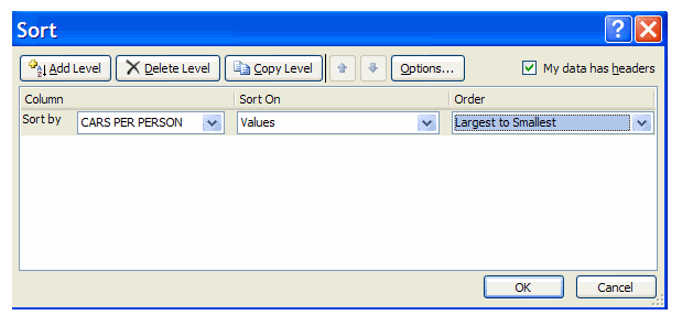
• Suppose we wish toorderthe newly created data in descending order by cars per person.

• Highlight cells A1:C6
• Choose the Data Tab and the Sort and Filter Group and Sort This opens the Sort Dialog box
• Sort by CARS PER PERSON from largest to smallest.

DELETE ROWS OR COLUMNS OF DATA

• In most cases we wish to delete an entire row or column. If you just highlight the row or column and hit the delete key then the contents disappear but the row or column (now blank) remains. Instead click on the shaded row number or column letter and then right-click and choose delete. Alternatively highlight the row(s) and column(s) to delete and then choose Edit | Delete and select delete all row or delete all column.

Charts

It can often be difficult to interpret Excel workbooks that contain a lot of data. Charts allow you to illustrate your workbook data graphically, which makes it easy to visualize comparisons and trends.

The Various Type of Charts

Identify Various Type of Charts

Types of charts are:

• Pie chart
• Line chart
• Column chart
• Bar chart
• Area chart
• Scatter chart

Create Charts

Create Charts

To insert a chart:

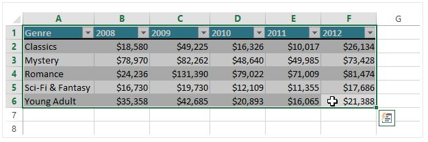
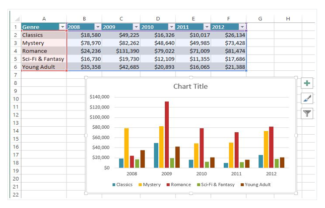
• Select thecellsyou want to chart, including thecolumn titlesandrow labels. These cells will be thesource datafor the chart. In our example, we'll select cells A1:F6.

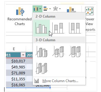
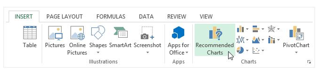
From the Insert tab, click the desired Chart command. In our example, we'll select Column.

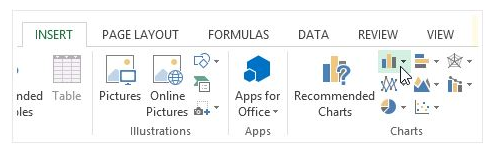
Choose the desired chart type from the drop-down menu.

The selected chart will be inserted in the worksheet.

If you're not sure which type of chart to use, the Recommended Charts command will suggest several different charts based on the source data.

Edit Charts

Edit Charts

Chart layout and style

• After inserting a chart, there are several things you may want to change about the way your data is displayed. It's easy to edit a chart's layout and style from the Design tab.
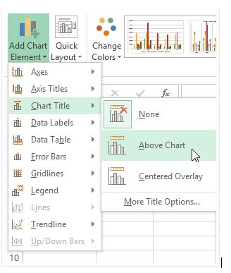
• Excel allows you to add chart elements —such as chart titles, legends, and data labels—to make your chart easier to read.
• To add a chart element, click the Add Chart Element command on the Design tab, then choose the desired element from the drop-down menu.

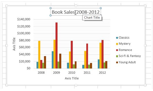
To edit a chart element, like a chart title, simply double-click the place holder and begin typing.

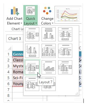
If you don't want to add chart elements individually, you can use one of Excel's predefined layouts. Simply click the Quick Layout command, then choose the desired layout from the drop-down menu.

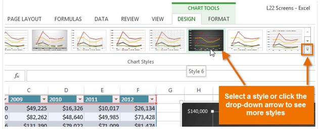
Excel also includes several different chart styles, which allow you to quickly modify the look and feel of your chart. To change the chart style, select the desired style from the Chart styles group

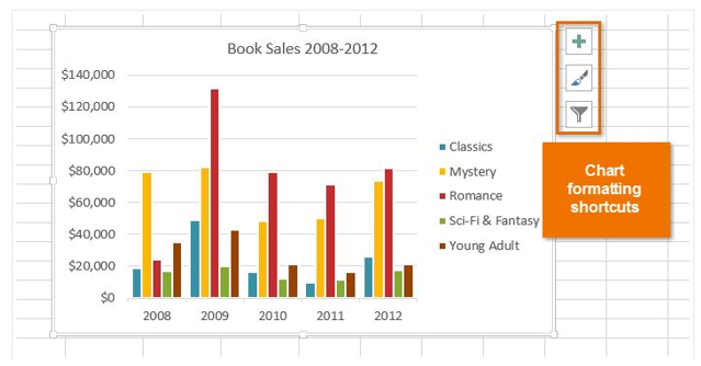
You can also use the chart formatting shortcut buttons to quickly add chart elements, change the chart style, and filter the chart data.

Other chart options

• There are many other ways to customize and organize your charts. For example, Excel allows you to rearrange a chart's data, change the chart type, and even move the chart to a different location in the workbook.

To switch row and column data:

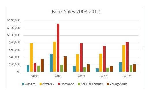
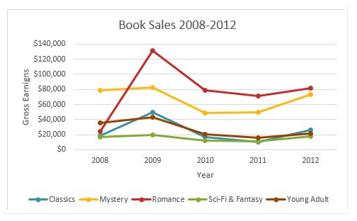
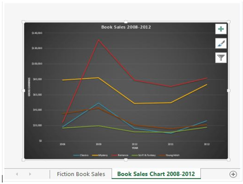
• Sometimes you may want to change the way chartsgroupyour data. For example, in the chart below, the Book Sales data are groupedbyyear, with columns foreachgenre. However, we could switch the rows and columns so the chart will group the databy genre, with columns foreachyear. In both cases, the chart contains the same data—it's just organized differently.

• Select the chart you want to modify.
• From the Design tab, select the Switch Row/Column command.

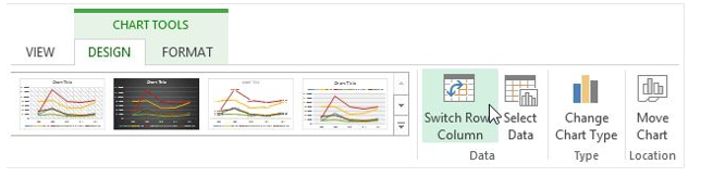
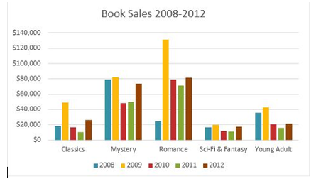
• The rows and columns will be switched. In our example, the data is now grouped by genre, with columns for each year.

To change the chart type

• If you find that your data isn't well suited to a certain chart, it's easy to switch to a new chart type. In our example, we'll change our chart from a Column chart to a Line chart.
• From the Design tab, click the Change Chart Type command.

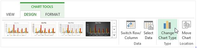
The Change Chart Type dialog box will appear. Select a new chart type and layout, then click OK. In our example, we'll choose a Line chart.

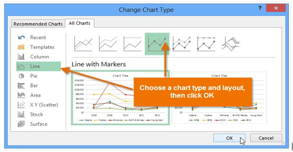
The selected chart type will appear. In our example, the line chart makes it easier to see trends in the sales data over time.

To move a chart:

• Whenever you insert a new chart, it will appear as an object on the same worksheet that contains its source data. Alternatively, you can move the chart to a new worksheet to help keep your data organized.
• Select thechartyou want to move.
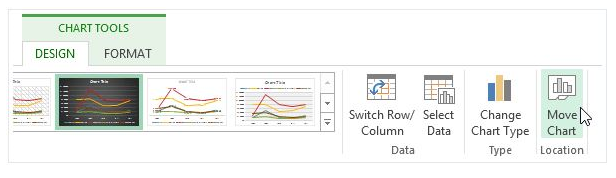
• Click the Design tab, then select the Move Chart command.

• The Move Chart dialog box will appear. Select the desired location for the chart. In our example, we'll choose to move it to a new sheet, which will create a new worksheet.
• Click OK.

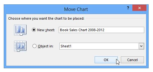
• The chart will appear in the selected location. In our example, the chart now appears on a new worksheet.

Printing a Worksheet

You can print entire or partial worksheets and workbooks, one at a time, or several at once. And if the data that you want to print is in a Microsoft Excel table, you can print just the Excel table. You can also print a workbook to a file instead of to a printer. This is useful when you need to print the workbook on a different type of printer from the one that you originally used to print it.

Help Facility

The Office Help Facility

Use Office Help Facility

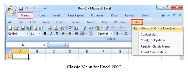
Help button on Classic Menus

• With Classic Menu for Excel 2007/2010/2013/2016 installed, you can click Menus tab to get back the classic style interface. The Help menu lies in the right most of the toolbar.

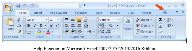
Help button on Ribbon Interface

• The Help button in Excel is too small that will be easily ignored. Actually the Help button stays in the top right corner of the window. The button looks like a question mark surrounded by a circle. The following picture shows its position. Or you can use the shortcut key F1 to enable the Help window.